HOW TO MAKE INFERENTIAL STATISTICS WITH SPSS
October 13 2018, By Chidi Rafael
When decisions or judgements are to be made from a study or a descriptive data, it is imperative to adopt various techniques for inferences.
One way to make inferences is by formulating a Hypothesis. A hypothesis may be needed in a study for users to decide appropriately on whether an assumption is true or false.
To make this tutorial simple and straight forward for a beginner, I will stick with these areas where Inferential Statistics could be applied in research. These four areas are:
- Relationships.
- Association.
- Correlation.
- Variance.
Before we go deep into these four major areas mentioned above, it is necessary to know the Decision Rule when Using the Statistical Package for Social Sciences (SPSS) for judgements.
Using a 95% Confidence Level, the decision is pegged at 0.05. (p =0.05). This simply implies that when p (the Significance level) is less than or equal to 0.05, we should accept (i.e. it is Significant Statistically).
On the other hand, when p is greater than 0.05, we should reject the hypothesis (i.e. it is not Significant Statistically).
The table below represents the Decision Rule:
Result |
Decision |
p< or = 0.05 |
Accept (Significant) |
p> 0.05 |
Reject (Not Significant) |
Figure 1.0
*This is dependent on a significance level of 0.05.
A) Relationships: Applying Linear Regression in SPSS
To measure relationship(s) between two or more variables linearly, we can use the Linear Regression. The example below illustrates how this can be applied using SPSS.
Illustration 1
The following data shows the Income and Expenditure pattern of Mr. Okoro from January to June 2018.
MR OKORO |
||
INCOME AND EXPENDITURE REPORT FROM JAN-JUNE 2018 |
||
MONTH |
INCOME (NGN) |
EXPENDITURE (NGN) |
JAN |
35,000 |
32,500 |
FEB |
50,000 |
43,000 |
MAR |
53,000 |
50,000 |
MAY |
61,000 |
58,000 |
JUNE |
74,000 |
73,000 |
Figure 2.0
Objective
To compute the data in Figure 2.0 in SPSS and test if there is a Significant Relationship between Income and Expenditure.
Solution to Illustration 1 Using SPSS
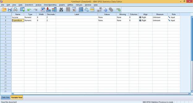
- Open the SPSS Software and click on Variable View

- Name your Variables (No spaces Accepted) as shown below:

Credit: IBM SPSS Statistics
- Click on Data View
 button to enter the values or results gotten from the study. See below:

Credit: IBM SPSS Statistics
- Click on Analyze > Regression > Linear.
- Move the Income Variable to the Independent(s) and Expenditure Variable to Dependent using the Arrow button

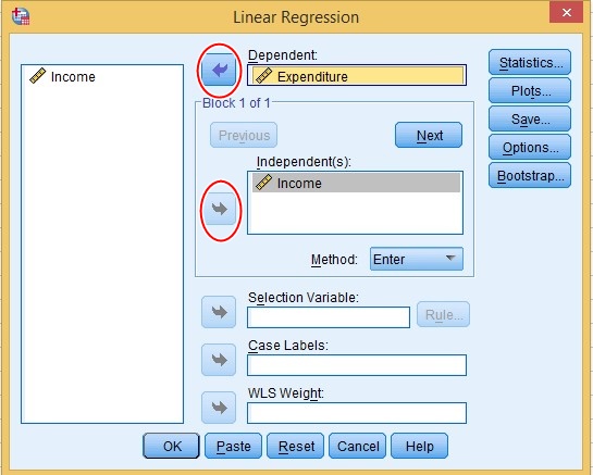
Credit: IBM SPSS Statistics
- Click OK
 for the result to display in the SPSS Output Screen.
Click to Download SPSS Software
Interpreting the Result
Our emphasis will be on 3 major tables:
- Model Summary.
- ANOVA.
- Coefficients.
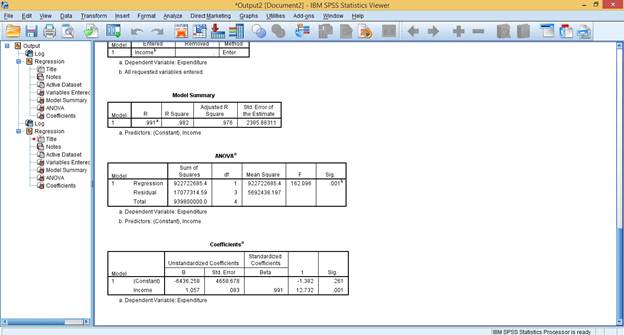
Credit: IBM SPSS Statistics
Model Summary
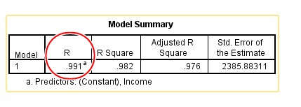
The model Summary shows the relationship between the variables. R of 0.991 shows the strength of the relationship between the Independent Variable/Predictor (Income) and the Dependent Variable (Expenditure) in Decimal or Percentage form.
From the above example, Income accounts for 0.991 or 99.1% change in Expenditure. In other words, 99.1% change in Expenditure can be explained by the Predictor (Income).
ANOVA
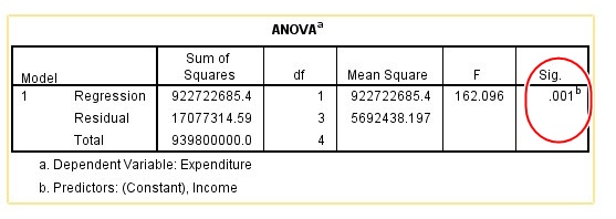
The ANOVA table is used to check for Fitness of data in the model. To decide whether there is a statistically significant relationship between variables, we will look at the heighted in the Sig. Column above.
The Sig. Column of 0.001 is less than 0.05 (See Figure 1.0 for Decision Rule). This implies that there is a Statistically Significant relationship between Income and Expenditure.
Coefficients
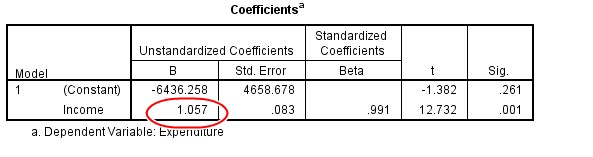
The Coefficients table provides us with information to predict Expenditure from Income.
The highlighted above shows that 1 unit increase in Income will result to 1.057 increase in Expenditure.
B) ASSOCIATIONS: APPLYING CHI-SQUARE IN SPSS
Chi-Square can be used to test for Association between two or more variables. The Chi-Squared test measures if there is a significant difference between Expected Frequency (EF) and the Observed Frequency (OF).
Illustration 2
A survey was conducted on the reading preference of Undergraduate Students in The University of Abuja. With a Sample Size (n) of 20, the following results were gotten:
Gender |
Preferred Reading Method |
Total |
|
Book |
Online |
||
Male |
3 |
7 |
10 |
Female |
6 |
4 |
10 |
|
|
Total |
20 |
Figure 3.0
Objective
From the above data in Figure 3.0, You are required to compute the results in SPSS and test for Association between Gender and Preferred Reading Method using Chi-Square.
Solution to Illustration 2 in SPSS
- Enter the Data (As shown in Figure 2.0) in the Data View
 as shown below:
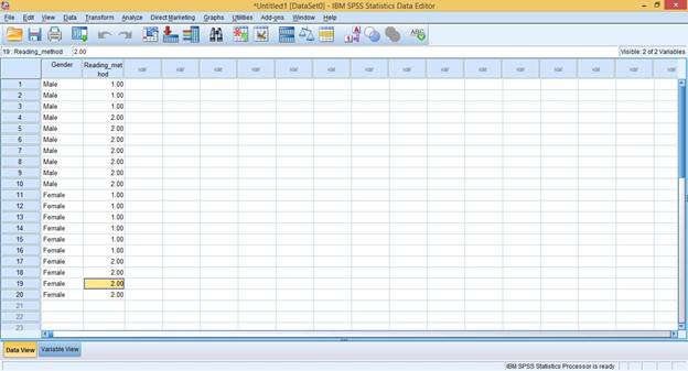
Credit: IBM SPSS Statistics
NOTE: A little Data Coding is required in the Variable View. Data Type for Gender should be changed to ‘String’, and ‘1’ should be used to represent ‘Book’, 2 should represent ‘Online’.
- Click on Analyze > Descriptive > Cross Tabs
- Use the Arrow Button
 to move the Gender Variable to Row(s) and Reading_Method Variable to Column(S).
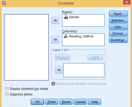
Credit: IBM SPSS Statistics
-
Click on the Statistics
 button. Select Chi-Square and Phi and Cramer’s V, then Click on Continue
  .
.
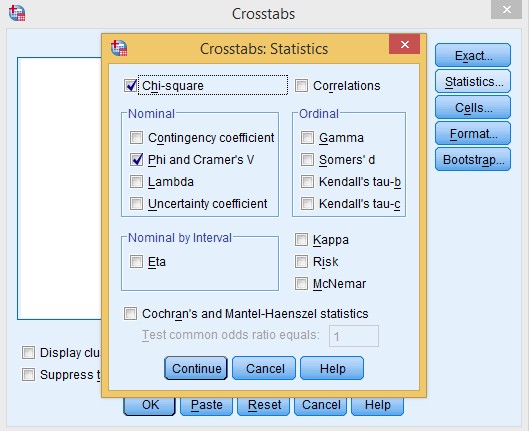
Credit: IBM SPSS Statistics
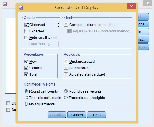
- Click on the Cells
 button. Select Observed, Row Column and Total. Click Continue
  .
.
Credit: IBM SPSS Statistics
- Finally, Click the OK
 button for the Result.
Credit: IBM SPSS Statistics
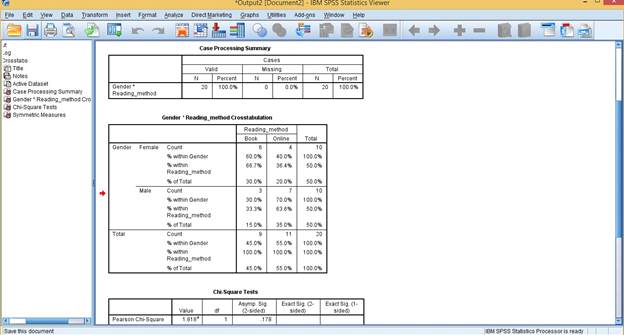
Interpreting the Result
The Crosstabulation Table
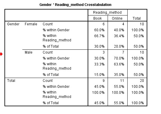
This table simply illustrates the frequency distributions of Gender Versus Reading Method Preferences of the Respondents used for the study.
Chi-Square Tests
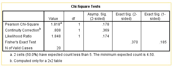
This is the most important table used for measuring Association between variables used for the study.
From the table, the Pearson Chi-Square (p) = 0.178. since p > 0.05, we can conclude that there is no Statistically Significant association between Gender and the reading preference of Undergraduates in the University of Abuja.
C) APPLYING CORRELATION IN SPSS
The Pearson Correlation test measures the strength and direction of two variables. We will use the illustration below to demonstrate this.
Illustration 3
The following data shows the Income and Expenditure pattern of Mr. Okoro from January to June 2018.
MR OKORO |
||
INCOME AND EXPENDITURE REPORT FROM JAN-JUNE 2018 |
||
MONTH |
INCOME (NGN) |
EXPENDITURE (NGN) |
JAN |
35,000 |
32,500 |
FEB |
50,000 |
43,000 |
MAR |
53,000 |
50,000 |
MAY |
61,000 |
58,000 |
JUNE |
74,000 |
73,000 |
Figure 4.0
Objective
You are to compute the data in Figure 4.0 using SPSS and test if there is a Significant Correlation between Income and Expenditure.
Solution to Illustration 3 in SPSS
- Properly Name your variables (Income and Expenditure) in the Variable View
 and Enter your data on the Data View
  as shown below:
Credit: IBM SPSS Statistics
- Click on Analyze > Correlate > Bivariate
- Use the Arrow button
 to move both variables to the Variables Box.
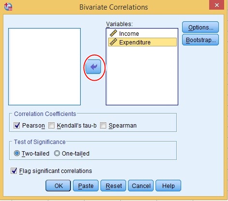
Credit: IBM SPSS Statistics
- Click OK

Interpreting the Result
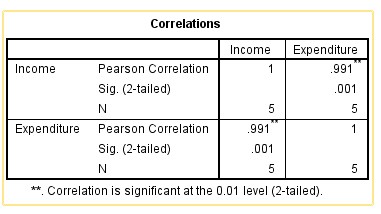
The table above presents a mix of the Pearson Correlation, the Significance Value (Sig.) and the Sample Size (N) in a matrix form.
The Pearson Correlation (r) = 0.991 with p = 0.001. This implies that there is a significant Correlation between Income and Expenditure, since p < 0.05.
D) TEST FOR VARIANCE: APPLYING ONE WAY ANOVA IN SPSS
One way to test for variance is through One-Way ANOVA. One-way ANOVA compares the means between two or more variables to test for a statistically significant difference.
One-way ANOVA is most suitable for testing variance between two or more unrelated groups.
Click to Download SPSS Software
Illustration 4
A Quiz was set for two groups (Male and Female) in a class to determine if there is a significant difference between Gender and Academic Performance. With a sample size(n) of 10, the results below were gotten.
Name |
Gender |
Score |
John |
Male |
20.01 |
Mark |
Male |
15.98 |
Andrew |
Male |
43 |
Peter |
Male |
21.4 |
Solomon |
Male |
32.4 |
Joy |
Female |
20.12 |
Amaka |
Female |
13.5 |
Rose |
Female |
56.1 |
Cynthia |
Female |
18.7 |
Emem |
Female |
45.2 |
Figure 5.0
Objective
You are Required to Compute the Data in Figure 5.0 using SPSS and test for Variance using the One-Way ANOVA.
Solution to Illustration 4 in SPSS
- Enter the data properly in SPSS. You Data View should look like this:
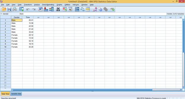
Credit: IBM SPSS Statistics
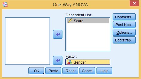
- Click on Analyze > Compare Means > One-Way ANOVA.
-
Use the Arrow Button
 to move the Dependent Variable (Score) to the Dependent List, and the Independent Variable (Gender) to the ‘Factor’ Field.
Credit: IBM SPSS Statistics
- Click on OK
 .
.
Interpreting the Result
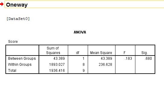
The ANOVA table represents the results between Groups and within Groups used for the study. p= 0.680 shows that there is no statistically significant difference between Gender and Academic Performance of students used for the study.
Click to Download SPSS Software
You may also like: Making Awesome Presentations│ Developing Outstanding Research Topics │How to Write an abstarct │How to Write a Project Proposal │How To Choose the Right Measurement Instrument